when do you sleep? learning a pattern of life from message timestamps
how a tiny probabilistic model can infer sleep, daily rhythm, and even rough timezone using nothing but message timestamps
find all the code here
given nothing but message timestamps, this program estimates when you sleep, when you wake up, and your rough timezone. for one user, it produces:
~ inferred timezone: UTC+3

+ typical schedule:
        - sleep: 23:52 -> 06:34  (≈ 8h 30m)
        - awake: 06:34 -> 23:52
        - variability: ±175m

+ activity profile (24h):
        ▁▁▁▁▁▁▁▁▅▇▅█▆▁▅▄▅▆▁▇▇▆▆▇
        |     |     |     |
        00    06    12    18

+ fingerprint:
        parcae:v1:AAAAAAAAAAAAAAAAAAAAAD0AWQA6AGMAQQAAADoAMAA6AEcAAABWAFUATgBMAFsAd__-D9QPqP12BPEBqwU=

~ based on 30 days of data
~ bin size: 15 minutes
people leave a strong daily signature in their activity: long stretches of silence, short bursts of messages, and a rhythm that repeats every 24 hours. over days and weeks, those gaps and bursts line up into a pattern. from that pattern, you can recover information such as their typical sleep and wake times, whether someone is active during the day or night, and even a rough estimate of their timezone.
how it works
the problem can be written in probabilistic terms. for each user, we observe a sequence of message timestamps. after binning time into fixed intervals, this becomes a binary time series:
each bin indicates whether at least one message occurred, and we model this sequence with a simple two-state hidden process: A (awake) and S (sleep).
the process tends to remain in the same state for long periods, producing many messages in A and few in S. the goal is to infer the most plausible hidden state sequence given the observations.
formally, this is a 2-state hidden markov model. for any candidate state sequence Z, its score is
the emission terms reward states that match the observed activity (messages while awake, silence while asleep), and the transition terms favor infrequent switching, producing long contiguous blocks.
rather than committing to a single explanation, we evaluate the total likelihood:
we repeat this computation for multiple timezone shifts φ by shifting the entire timeline by φ and computing its likelihood P(O_φ). the shift that maximizes this likelihood is taken as the most plausible timezone:
finally, with the best shift fixed, we decode the single most likely state sequence:
this yields three outputs from timestamps alone: an estimated timezone, a segmentation into sleep and wake periods, and a compact summary of the user’s daily rhythm.
implementation
data
the first step was to get some real-world data.
for this, I exported two very large and very active discord servers, specifically their “general” text channel. this yielded a dataset of about 542,382 message timestamps across a few hundred users.
after grouping by user and discarding users with very little activity, i ended up with 213 users, each with on the order of months of activity.
update as of 2026-01-30: 886,854 timestamps over three discord servers across 352 usersbinning
raw timestamps are not very convenient to work with directly, so the first step is to bin time. i chose 15-minute bins which is large enough that “awake” bins usually contain activity and not so small that everything becomes noise.
for each user, i take their first and last timestamp, create a regular grid of 15-minute bins covering that span, and set:
o_t = 1 # if at least one message falls in that bin
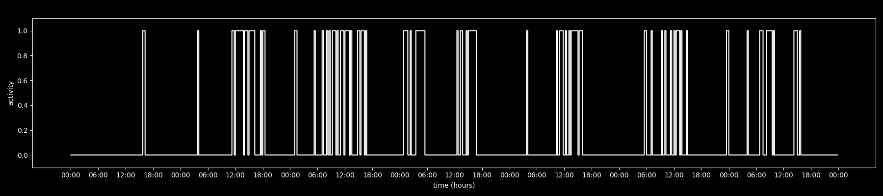
o_t = 0 # otherwisethis turns each user into a binary time series like: 000000000011111111111111000000000000000000111111111...
plotted over time, it looks like this:
start = timestamps.min().floor("D")
end = timestamps.max().ceil("D")

bin_delta = timedelta(minutes=BIN_MINUTES) # BIN_MINUTES=15
n_bins = int((end - start) / bin_delta) + 1

bins = numpy.zeros(n_bins, dtype=numpy.uint8)
indices = ((timestamps - start) / bin_delta).astype(int)

bins[numpy.unique(indices)] = 1
training the model
the model itself is just a 2-state hidden markov model with state 0 representing one activity regime and state 1 representing the other.
here denotes the hidden state at time bin (sleep or awake).
we do not tell it which one is “sleep” and which one is “awake”. it discovers that on its own.
the observation model is categorical:
and the transition model is:
after training the model on the full dataset, we can just print out the learned parameters.
this is what i got*:
[=] startprob: [0.97684097 0.02315903]
[=] transmat: [[0.98054312 0.01945688]
 [0.20483654 0.79516346]]
[=] emissionprob: [[9.99999819e-01 1.80571797e-07]
[5.62094722e-01 4.37905278e-01]]remember that one state will end up meaning “sleep”, the other will end up meaning “awake”, but we never tell the model which is which. we can interpret these numbers in plain english:
[=] emissionprob: [[9.99999819e-01 1.80571797e-07]
 [5.62094722e-01 4.37905278e-01]]
this means that state 0 emits 0 (no message) almost all the time
state 0 emits 1 (a message) essentially never
state 1 emits 0 about 56% of the time
state 1 emits 1 about 44% of the time
so one state is almost always silent and the other is roughly half the time active, it is very clear which one corresponds to sleep and which one corresponds to awake.
[=] transmat: [[0.98054312 0.01945688]
 [0.20483654 0.79516346]]
this means that if you are in state 0, you stay there with ~98 probability per 15-minute bin. if you are in state 1, you stay there with ~80 probability per 15-minute bin.
meaning both states are “sticky” but the silent (sleep) state is much “stickier” which produces long uninterrupted sleep blocks and somewhat more fragmented awake periods.
inference: finding the timezone
for a new user, the model is already trained. now we just want to answer: which shift of the timeline makes this data look most like it came from a human with one long sleep per day?
so for each candidate timezone offset φ (e.g., from -12 to +12), we shift the binned sequence up by φ and compute its total likelihood using this forward algorithm:
we then pick the one that scored the highest:
this is extremely simple and extremely effective.
best_phi = 0
best_score = -numpy.inf

for phi in tz_range: # tz_range=(-12, 13)
        shift_bins = int(phi * bins_per_day / 24) # for 15 minutes, bins_per_day=96
        bins_phi = numpy.roll(bins, shift_bins)

        score = _forward_log(
                bins_phi,
                self.log_transmat,
                self.log_emissionprob,
                self.log_startprob,
        )

        if score > best_score:
                best_score = score
                best_phi = phi # best_phi (φ*) being the most likely timezone offset
where _forward_log is
and implemented as
def _forward_log(obs, log_trans, log_emit, log_init):
    T = len(obs)
    alpha = numpy.zeros((T, 2))

    alpha[0] = log_init + log_emit[:, obs[0]]

    for t in range(1, T):
        for j in range(2):
            alpha[t, j] = log_emit[j, obs[t]] + _logsumexp(
                alpha[t - 1] + log_trans[:, j]
            )

    return _logsumexp(alpha[T - 1])
decoding sleep and awake
once we have the best shift φ*, we run Viterbi to get the single best state sequence:
from this we extract contiguous blocks: sleep blocks and awake blocks. this is the model’s full explanation of the timeline.
shift_bins = int(best_phi * bins_per_day / 24)
best_bins = np.roll(bins, shift_bins)

states, _ = _viterbi(
        best_bins, self.log_transmat, self.log_emissionprob, self.log_startprob
)

sleep_blocks = []
awake_blocks = []

current_state = states[0]
block_start = 0

for i in range(1, len(states)):
        if states[i] != current_state:
                (sleep_blocks if current_state == self.sleep_state else awake_blocks).append((block_start, i))

        block_start = i
        current_state = states[i]
def _viterbi(obs, log_trans, log_emit, log_init):
T = len(obs)
dp = np.zeros((T, 2))
back = np.zeros((T, 2), dtype=np.uint8)
dp[0] = log_init + log_emit[:, obs[0]]
for t in range(1, T):
for j in range(2):
scores = dp[t - 1] + log_trans[:, j]
k = np.argmax(scores)
dp[t, j] = scores[k] + log_emit[j, obs[t]]
back[t, j] = k
last = np.argmax(dp[T - 1])
best = dp[T - 1, last]
path = np.zeros(T, dtype=np.int8)
path[T - 1] = last
for t in range(T - 2, -1, -1):
path[t] = back[t + 1, path[t + 1]]
return path, bestsummarizing and extracting daily features
the raw sleep and awake blocks are useful internally, but they are not very readable on their own. the CLI first converts them to local time and summarizes each day’s longest sleep interval into a typical daily schedule.
from the same decoded states we also compute a compact set of daily features. these include an averaged 24-hour activity profile, typical sleep start and end times estimated with circular statistics, and summary measures of sleep duration such as mean, variability, and median length.
these features power the printed schedule and serve as the inputs to the fingerprint below.
fingerprint
the CLI also emits a small fingerprint string:
parcae:v1:AAAAAAAAAAAAAAAAAAAAAD0AWQA6AGMAQQAAADoAMAA6AEcAAABWAFUATgBMAFsAd__-D9QPqP12BPEBqwU=this encodes the features described above by concatenating, quantizing, and base64-encoding them into a short string. two fingerprints can be compared directly:
parcae compare parcae:v1:<fp1> parcae:v1:<fp2>the tool computes cosine similarity between the vectors. high similarity suggests the same person or very similar schedules, and low similarity suggests different routines.
this makes it possible to cluster similar users, detect alternate accounts, and track how someone’s schedule changes over time.
limitations
this is a small, exploratory experiment. the model is intentionally simple (two states, 15-minute bins). it cannot represent naps, split sleep, shift work, irregular schedules, or people who are frequently idle while awake.
results depend heavily on the behavior of the person, and this is best viewed as a proof of concept: it shows that there is a surprising amount of structure in timestamp-only data, and that a very small probabilistic model can recover some of it, but it is not precise.
naming
I decided to name this project “Parcae” after the roman myth, they are the greek equivalent of the “Moirai” however that name was already taken on PyPi.
according to the myth, the name of the three Parcae are Nona (the greek Clotho), Decima (the greek Lachesis), and Morta (the greek Atropos).
nona spun the thread of life (this represents the beginning of a person’s life). decima measured the thread of life (this represents the length and structure of that life). morta cut the thread of life (this represents the end of that life, or a final boundary).
the metaphor maps nicely on what the project is trying to do: take a long, continuous timeline of activity, figure out where it meaningfully begins (waking up) and ends (sleep), and then describe the structure in between. this ends up corresponding to things like daily cycles, active periods, and sleep windows.